1.5 Fractional Systems
It follows from Equation (15) that the loop transfer function is not a rational function. We illustrate this with an example.
Example
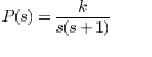
Consider a process with the transfer function
Assume that we would like to have a closed loop system that is insensitive to gain variations with a phase margin of 45. Bode�s ideal loop transfer function that gives this phase margin is  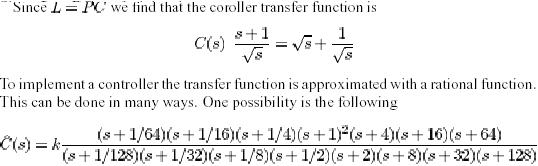
Where the gain k is chosen to equal the gain of Notice that the controller is composed of equal length having
slopes 0,+1 and -1 in the Bode diagram. Figure 6shows the Bode diagram for the loop transfer function. The figure shows that the phase margin will be close to 45 with a tolerance of less than 2 for a gain variation of 3 orders of magnitude. With a tolerance of 5 we can even allow a gain variation of 4 orders of magnitude. The range of gains of gains can be extended by making the controller more complex. Even if the closed loop system has the same phase margin when the gain changes the response speed will change with the gain.
The example shows that robustness is obtained is obtained by increasing controller complexity. The range of gain variation that the system can tolerate can be increased by increasing the complexity of the controller.
Fractional system did not receive much attention after Bodes work. In the 1990s there was however a resurgence
in the interest of fractional systems, see. G.[53,54,55,56,57] . oustaloup coined the acroyme CRONE from the French commande Robuste d�Ordre non Entire (Robust Control of Fractional Order)for his controller.
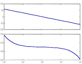
Fig. 6: Bode diagram of the loop transfer function obtained by approximating the fractional controller with a rational transfer function.
Two Degree of Freedom Systems (2DOF)
The system in Figure 2 is a system with error feedback because the controller acts on the error e=r �y which is the difference between the set point and the output. There are Significant advantages in having control systems with other configurations. An example of such a system is shown in Figure 7. in this system the set point is fed through a model before it is compared with the process output. There is also a feedforward link which essentially is a combination of the model and the inverse process model or an approximate inverse. Ideally the feedforward signal uff generates a signal which when applied to the process procures the ideal output inresponse to set point changes. The feedback controller which acts on the error will only make some corrections if there are deviations from the ideal behavior.
A system with error feedback only is called a system with one degree of freedom. The system in figure 7 is called a system with two degrees of freedom (2DOF) because the signal paths from the set point to the control signal is different from the signal path
|