| Transfer Functions |
What can you learn from the transfer function?
Knowing the transfer function of a system (controlled or uncontrolled) allows you to infer many things about its performance. The most important things you can learn from the transfer function, H (s) are summarized here:
1. stability
Start with the output of a continuous system in the complex frequency (-s) domain:

Notice that the inverse laplace transform o (t) the output as a time- function will be a sum of exponentials with each term looking like
 This says that regardless of the mature of the input if the system has any poles that lie in the right half of the complex plane the output will contain terms that grow without limit
Therefore, any continuous system with poles in the right half of the complex plane is unstable, also in order to determine if a system is unstable, all you need to do is to find its poles, provided you can find the system poles, any other alternative method of determining stability is unnecessary the GSim Compute poles. Vi will compute the poles of any transfer function for which the a � coefficients are known.
2. Relative importance of poles: the dominant- pole approximation
The residue-pole form of 0(s), above, lets you rank the relative contribution of each pole two different ways:
- reative magnitude, determined by the relative magnitude of each residue, a
- decay rate determined by the pole�s horizontal location in the complex plane
outputs from poles located far to the left in the complex plane decay so quickly that they are of lesser importance relative to outputs arising from poles further to the right in the complex plane. it many cases you can approximate the transfer function of a high- order system with a lower-order one containing only the dominant poles (those located closest to the imaginary axis)
3 steady- state errors
A control system designer who is not too demanding might be happy with a control system that finally produces an output exactly as commanded by the control signal �if you wait long enough � this crude specifications is usually only a starting points but is you usually part of the list of specs the designer must meet.
If we define �error� as the difference between command and actual system output.
Then its LaPlace transform is
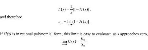
 the final value theorem for laplace transforms says that the final value theorem for laplace transforms says that

For any function of time, e(t) clearly, e depends on r(t) so let�s consider some special cases of practical interest:
a) steady- state error for a step a step function input, R(s) =1/s:Zero steady- state error in this case means that, given enough time, the system should finally track a command signal exactly after the command signal changes discontinuously to a new constant level . in this case.
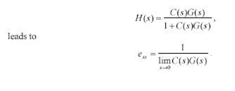
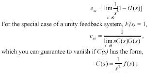
 for zero steady-state error limit should be unity. For a controlled system with unity feedback and cascade compensation, C(s). only ,I .e F (s) =1 using the transfer function,

This result is important for the design guidance it provides: since in principle you can design C(s) however you wish , you guarantee zero steady-state error by putting a pole in C(s) at �o such as

Where F(s) is any other rational polynomial function of s classical control texts call this a type 1system since 1/s is the laplace transform corresponding to integration you can think of this condition as a reqyurement for integrating the error signal e(t). if the error is
 Where f(s) is any other rational polynomial function of s classical control texts call this a type 2 system since 1/s is the laplace transform corresponding to integration, you can think of this condition as a requirement for integrating the error signal , e(t), twice.
These arguments can be extended to specifications requiring the tracking of command signal with constant accelerations and even higher time derivatives.
4. Response of controlled systems to disturbance
A control system engineer�s life would be simple indeed if the only inputs to systems were the command signals, r(t). a more realistic view of a controlled system in the s-domain is shown below including:
- disturbance d(s) at the input to the plant
- disturbance D(s) at the output to the plant
- noise N(s) in the feedback loop
this system is linear so you can treat these disturbances as additional inputs and use superposition. To help you use superposition correctly, you might consider breaking the feedback loop and an artificial �input� identical to the output 0(s), as show here
|

