The
37% Method
This gives us the first method for finding
a time constant. Here is the method.
-
Determine the initial
value of the variable, x(0) in the above.
-
Determine the time when
the variable has decayed to 37% of the initial value.
-
That time is the measured
time constant.
That is a simple method that can be applied
to numerous situations. You need to note the following.
-
You need a response that
dies out to zero. If you have a response that has the right shape,
but which does not die out to zero, then you may have to redefine a component
of the response in order to meet this requirement.
-
The method depends upon
the value of the response at only one point. In essence, you throw
away all of the data that you have except for the starting value and the
37% value.
The
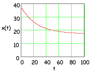
first note above has some implications. Here is a response that exhibits
time constant behavior.

This response does not decay to zero.
However, it does apparently decay to a value of 17, so if you subtracted
17 from the response you would get a response function that did decay to
zero. That might make some sense physically in many situations.
For example, the plot above might be the temperature above ambient (in
Celsius degrees) and the temperature rise above ambient would fall to zero
as the temperature fell to ambient in a thermal system. Look for
situations like that.
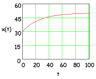
The same kind of reasoning would also apply to finding time constants from
step responses. Here is a step response.

Here the steady state is 50, and you could
take the difference between the steady state (50) and the response.
That difference decays to zero as the response approaches the steady state,
and that gives you the kind of function that you want.
Here is the method.
-
Determine the initial
slope of the variable, x(0) in the above.
-
Determine the time when
the variable would have decayed to zero if the initial rate of decay (slope)
had continued.
-
That time is the measured
time constant.
You need to note the following.
-
You do not need a response
that dies out to zero. If you have a response that decays to some
non-zero final value, just extend the initial slope line until the extended
line hits the final value.
-
The method depends upon
the slope of the response at only one point. In essence, you throw
away all of the data that you have except for the starting value and the
initial slope.
The
Initial Slope Method
There
are other methods that you can use. One other method usese the initial
slope of the response. Consider the equation for the response curve.
x(t) = x(0)e-t/t
The slope is given by:
dx(t)/dt = [-x(0)/t]e-t/t
Interestingly, if the
response continued to decay at this rate - and we know that it doesn't
- the response would decay to zero in t
seconds. Since the rate of change is -x(0)/t, if it continued
t
for seconds the total change would be -x(0), which would bring the response
to zero.
The implications of the argument above are that you can draw a line from
the initial point at the initial slope and check where that line intersects
the final value, and the time when that happens is the time constant.
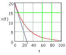
That is better when you have a visual representation. Here is a plot.

In this plot, the initial
slope has been extended (blue line) and intersects the final value (0)
at about 25 seconds, so the time constant would be 25 seconds.
The
Logarithmic Method
There
are other methods that you can use. Both of the previous methods
really depend upon values at a single time. There is another method
that uses all of the data. Consider the equation for the response
curve.
x(t) = x(0)e-t/t
Take the logarithm
of the response curve and we have the following.
ln[x(t)] = ln[x(0)]
- t/t
This is the equation
of a straight line when plotted against t. That leads us to the following
strategy.
-
Take a set of data at
different times. That data set would be x(tk) and
would comprise all of the values and all of the times.
-
Plot the values of the
data, x(tk), against the times, tk.
That should give you a straight line.
-
Determine the equation
of the line.
Note the following about
this method.
-
This method uses all of
the data.
-
If the data is noisy,
you can use regression to get the straight line parameters (slope and intercept).
-
You must (repeat MUST)
have data that decays to zero. If you do not have data that decays
to zero, see the note above about creating a set of data that decays to
zero by extracting the essential part of the data from the data set.
What
happens if you don't have a decaying exponential? In that case, you
need to isolate the decaying exponential that is buried in the data.
Here is an example.

In this response, the data does not decay to
zero. However, if you take the following steps, you can get a data
set that you can use with this method.
-
First, determine the steady
state. In real data sets you will have to make the best estimate
you can.
-
Secondly, subtract the
data from the steady state value you determined in the first step.
-
If the data can be put
into a spreadsheet that's an easy step.
-
You subtract the data
from the steady state so you can get numbers that are all positive so that
you can take a logarithm of your result in this step.
-
Finally, you have some
exponentially decaying data. Take the logarithm and you should see
a straight line. You might have to adjust the steady state value
a little in either direction to see what gives you the best straight line.
|

