Taylor Series | Complex Analysis | Mathematics | GATE Material | GATE Papers | GATE Preparation

Taylor Series

Taylor Series

Taylor Series.

Theorem 8.1.1 Let be a function analytic at a point . Denote by the largest circle centered at such that is analytic at all the points interior to , and let

be its radius. Then there exists a power series $\underset{k \geq 0}{\sum} a_k (z-z_0)^k$ which converges to in .

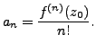
This series is unique; it is called the Taylor series of at . The cofficients of this series are determined by the following formula:

$\displaystyle a_n = \frac {f^{(n)}(z_0)}{n!}.$

The Taylor series of a function about 0 is called the Maclaurin series of .

Example 8.1.2 (Maclaurin series)

$e^z = 1 + z + \frac {z^2}{2!} + \frac {z^3}{3!} + \frac {z^4}{4!} + \dots = \underset{n=0}{\overset{+ \infty}{\sum}} \frac {z^n}{n!}$ .
$\cos z = 1 - \frac {z^2}{2!} + \frac {z^4}{4!} - \dots =\underset{n=0}{\overset{+ \infty}{\sum}} (-1)^n\frac {z^{2n}}{(2n)!}$ .
$\sin z = z - \frac {z^3}{3!} + \frac {z^5}{5!} - \dots = \underset{n=0}{\overset{+ \infty}{\sum}} (-1)^n\frac {z^{2n+1}}{(2n+1)!}$ .
$\cosh z = 1 + \frac {z^2}{2!} + \frac {z^4}{4!} + \dots = \underset{n=0}{\overset{+ \infty}{\sum}}\frac {z^{2n}}{(2n)!}$ .
$\sinh z = z + \frac {z^3}{3!} + \frac {z^5}{5!} + \dots =\underset{n=0}{\overset{+ \infty}{\sum}} \frac {z^{2n+1}}{(2n+1)!}$ .
$\frac {1}{1-z} = 1 + z + z^2 + z^3 + z^4 + \dots = \underset{n=0}{\overset{+ \infty}{\sum}} z^n$ .
$\log (1+z) = z -\frac {z^2}{2} + \frac {z^3}{3} - \frac {z^4}{4} + \dots = \underset{n=1}{\overset{+ \infty}{\sum}} (-1)^{n+1} \frac {z^n}{n}$ .
$(1+z)^{\alpha} = 1 + \alpha z + \frac {\alpha (\alpha -1)}{2!} z^2 + \frac {\alpha (\alpha -1)(\alpha -2}{3!} z^3 + \dots$ .

How to compute quickly a Taylor series expansion?

Derive term-by-term the Taylor series of about to get the Taylor series of about the same point. The radius of convergence of both series is the same.
The Taylor series of is the sum of the Taylor series of and of .
The Taylor series of is the product of the Taylor series of and of .
If $g(z_0) \neq 0$ , the Taylor series of is the quotient of the Taylor series of by the Taylor series of , according to increasing power order.

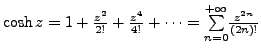
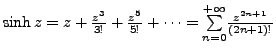
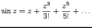
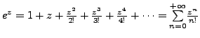
Example 8.1.3 Compute the Maclaurin series of $f(z)=\sin z \cdot e^z$ . Using 1.2, we have:

$\displaystyle \sin z \cdot e^z$	$\displaystyle = \left( z - \frac {z^3}{3!} + \frac {z^5}{5!} - \dots \right) \left( 1 + z + \frac {z^2}{2!} + \frac {z^3}{3!} + \frac {z^4}{4!} + \dots \right)$
$\displaystyle \quad$	$\displaystyle = z +z^2+\frac {z^3}{3}-\frac {z^5}{30}-\frac{z^7}{630}+\dots$

We can use Taylor series in order to find limits:

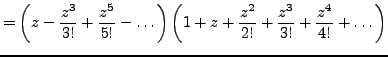
Example 8.1.4 Let $f(z)= \frac {e^z-1}{\sin z}$ . We wish to compute $\underset{z \rightarrow 0}{\lim} f(z)$ .

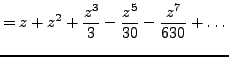
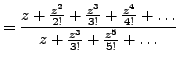
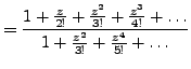
Using 1.2, we get:

$\displaystyle f(z)$	$\displaystyle = \frac {z + \frac {z^2}{2!} + \frac {z^3}{3!} + \frac {z^4}{4!} + \dots} {z + \frac {z^3}{3!} + \frac {z^5}{5!} + \dots}$
$\displaystyle \quad$	$\displaystyle = \frac {1 + \frac {z}{2!} + \frac {z^2}{3!} + \frac {z^3}{4!} + \dots} {1 + \frac {z^2}{3!} + \frac {z^4}{5!} + \dots}$

Therefore $\underset{z \rightarrow 0}{\lim} f(z)=1$ .

The following result is a consequence of Thm 3.5 and Thm 3.7.

Proposition 8.1.5 Let be a function analytic on a neighborhood of .

We get the Taylor series expansion of by differentiating term-by-term the Taylor series expansion of .
If the Taylor series expansion of is known, we get the expansion of by integrating term-by-term the Taylor series expansion of (take care of the additive constant of integration!)

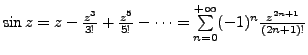
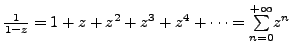
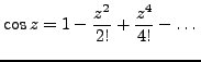
Example 8.1.6 In 1.2, we saw that

$\displaystyle \sin z = z + \frac {z^3}{3!} + \frac {z^5}{5!} + \dots$

By term-by-term differentiation, we have:

$\displaystyle \cos z = 1 - \frac {z^2}{2!} + \frac {z^4}{4!} - \dots$

and this fits 1.2.

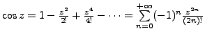
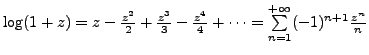
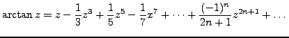
Example 8.1.7 Let $f(z)=\frac {1}{1+z^2}$ . The MacLaurin series of

is:

$\displaystyle f(z)=\frac {1}{1+z^2} = 1-z^2+z^4-z^6 + \dots + (-1)^nz^{2n} + \dots$

By integration term-by-term, we have:

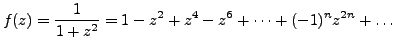
$\displaystyle \arctan z = z - \frac 13 z^3 + \frac 15 z^5 - \frac 17 x^7 + \dots + \frac {(-1)^n}{2n+1} z^{2n+1} + \dots$

Important remark: When we studied power series over the reals we had a surprise: the convergence domain of a power series is not always obvious.

Take . This function is defined over $\mathbb{R}-\{ 1 \}$ . Its first MacLaurin expansions are given by:

$\displaystyle P_1(x)$	$\displaystyle = 1+x$
$\displaystyle P_2(x)$	$\displaystyle = 1+ x + x^2$
$\displaystyle P_3 (x)$	$\displaystyle = 1+ x + x^2+x^3$
$\displaystyle P_4 (x)$	$\displaystyle = 1+ x + x^2+x^3+x^4.$

The graphs of and of these approximations are displayed in Figure 1.

**Figure 1:** First approximations of a given function.
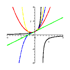$\begin{figure}\centering \mbox{ \epsfig{file=Taylor-CV-01.eps,height=6cm} } \end{figure}$

It seems that the visualization shows that the successive approximations tend to the original function only for . The condition for a geometric sequence to be convergent supports this impression. First of all, the function is not defined at 1 (where it has a singular point) and this point acts as a "barrier". But, does the power series make sense out of the interval ? Actually not in our frame of study. Maybe in other frames.

Now take 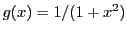. It is obtained by the substitution of instead of . The first MacLaurin expansions are given by:

$\displaystyle P_1(x)$	$\displaystyle = 1-x^2$
$\displaystyle P_2(x)$	$\displaystyle = 1-x^2 + x^4$
$\displaystyle P_3 (x)$	$\displaystyle = 1-x^2 + x^4-x^6$
$\displaystyle P_4 (x)$	$\displaystyle = 1-x^2 + x^4-x^6+x^8.$

The graphs of and of these approximations are displayed in Figure 2.

**Figure 2:** First approximations of a given function.
$\begin{figure}\centering \mbox{ \epsfig{file=Taylor-CV-02.eps,height=6cm} } \end{figure}$

We have here the same visual impression: the MacLaurin series tends to the given function for . But for the function , -1 and 1 are not points of discontinuity. So, what happens?

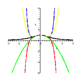
Passing to the complex setting, consider the function of the complex variable given by . It is defined over $\mathbb{C} - \{ -i, i \}$ . The corresponding MacLaurin series is given by and is convergent for in the open unit ball centered at the origin, i.e. on the largest ball centered at 0 at not touching the two points where fails to be defined

**Figure 3:** The largest ball for the function to be defined.
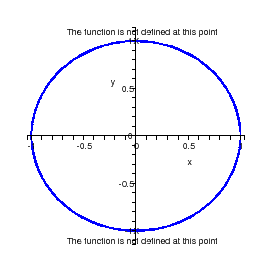$\begin{figure} % latex2html id marker 3455 \centering \mbox{ \epsfig{file=Non-definition-points-01.eps,height=6cm} } \end{figure}$

This example shows the importance of working in a complex setting. Without exaggeration, we could say that the complex setting is "more natural" than the real one.