The Fundamental Theorem of Linear
Programming
Having established all the necessary concepts and properties of the solution
space of n-var LP's, we are now ready to discuss the Fundamental Theorem
of Linear Programming. This theorem can be stated as follows:

Proof (Sketch): We establish the validity of Theorem1,
through a series of observations:
- First notice that according to the previous discussion, the feasible
region of an LP is a polytope, and thus, convex.
- Furthermore, since we assume that the LP has an optimal solution, let
 denote such an optimal point. The optimal objective value will be denoted by
 .
.
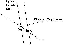
- Then notice that point
 cannot be interior to a line segment that is not perpendicular to the
direction of improvement to the ``isoprofit'' hyperplanes - w.l.o.g.,
let's assume a maximization LP for our discussion - defined by vector
 . Otherwise, by moving on this line segment in the direction of improvement
of the ``isoprofit'' hyperplanes,we would be able to obtain another point
 of the feasible region, such that
 . But this contradicts the assumption that
 is an optimal point. Figure9
depicts this argument.

Figure 9: Why an optimal solution to an LP cannot be
interior to a line segment not perpendicular to the direction of improvement
of the "isoprofit" hyperplanes
- However, point
 can be interior to a line segment of the feasible solution space which is
perpendicular to the direction of improvement of the optimal ``isoprofit''
hyperplane. This, in fact, corresponds to a situation of many optimal
solutions. In this case, notice that this line segment must have at least
one end
 defined by the fact that one (or more) additional constraint is binding at
this point. Otherwise, the problem is ill-posed, since we can vary some
variable(s) at will over
 with this variation affecting neither the constraints nor the objective.
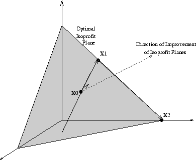
- Hence,
 , being on the optimal ``isoprofit'' hyperplane, is another optimal point at
which an additional constraint is binding. Then, there are two
possibilities: (i)
 is an extreme point of the feasible region, in which case we are done, or
(ii)
 is interior point to another line segment lying in the optimal ``isoprofit''
hyperplane
 , which binds, however, an additional constraint, compared to point
 . In this case, repeating the argument above, we establish the existence of
another end point
 , determined by the binding of at least one more constraint. Then, we repeat
the entire argument for
 , and so on. Figure10
depicts this part of the proof.

Figure 10: Identifying an optimal extreme point on the
optimal isoprofit hyperplane
- Finally, notice that every time we bind an additional constraint, we
restrict the (sub-)space of optimal solutions considered by one ``degree of
freedom''. Since an n-dim space has n ``degrees of freedom'',
the number of end points visited in the argument above before we find one
that it is an extreme point is finite. Thus, this last observation
establishes the existence of an optimal extreme point for the case of many
optimal solutions, and the proof is complete.
The discourse of the previous proof has also revealed a very important
property of extreme points: At these points, the number of binding constraints
is such that it allows zero ``degrees of freedom'', or, in other words,
these constraints define the point uniquely. Starting from this
observation, in the next section we provide a series of algebraic
characterizations of the extreme points, which will eventually allow us
to analytically manipulate the set of extreme points of an LP, in the context of
the Simplex algorithm. As it has been previously mentioned, this algorithm
exploits the result stated in the Fundamental Theorem above, by
limiting the search for an optimal solution over the set of extreme points of
the polytope defining the LP feasible region. In the next section, we shall show
that this set is finite and discrete, so it can even be
exhaustively enumerated. Simplex algorithm provides an efficient way to search
this set.
|

