| Model Uncertainty and Robust Control |
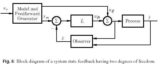
Robustness
In the model (20) it is natural to describe model uncertainties as variations in the elements of the matrices A,B and C. this is , however, a very restricted class of perturbations which does not cover neglected dynamics or small time delays such uncertainties are easier to describe in the frequency domain. The LQG theory was also criticized heavily by classic control theorist because it did not take robustness into account, see [25].
Very strong robustness properties could be established when all states were measured. In this case the system has a phase margin of 60 and infinite amplitude margin, see [42] which indicates a very good robustness.
The nice robustness properties of system with state feedback do not hold for systems with output feedback. Nice counterexamples were given in the paper [15]. For systems with output feedback it was attempted to recover the robustness of full state feedback making very fast observers. This approach led to a design technique called loop transfer recovery, see [18].
The only formal requirements on the system to be controlled in state-space theory is that the system is observable and controllable. There are no consideration of right half plane poles and zeros or time delays. Because of this it is necessary to investigate the robustness of the design and to make appropriate modifications to achieve good robustness. We use an example to illustrate what happens if this is not done.
Example: A fast system with a low bandwidth
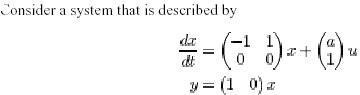 The system is controllable if a=1. we will assume that a=-10. the system is of second order and one state variable is measured directly. The system can be controlled with an observer of first degree. The closed loop system is then of order 3. we assume that a state feedback and an observe is designed so that the closed loop systems is
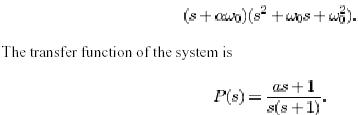 To obtain a fast closed-loop system we choose w=10 and a=1. straightforward calculations show that the controller has the transfer function
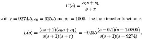 The process pole at s= -1 is almost canceled by the controller zero at s= -s1/s0= -1.0805. the Bode diagrams of the loop transfer function is shown in figure 9.
The loop transfer function has a low frequency asymptote that intersects the line log/L()| =0at w = - 1/a, i.e. at the slow unstable zero. The magnitude then becomes close to one and it remains so until the break point at w= r the controller pole. The phase is also close to � 180 over that frequency range which means that stability margin is very poor. The crossover frequency is 6.58 and the phase margin is . the maximum sensitivities are M=678and M=677 which also shows that the system is extremely sensitive. The slope of the magnitude curve at crossover is also very small which is another indication of the poor robustness of the system.
|