Nonlinear Model Predictive Control
Principles, Mathematical Formulation and properties of Nonlinear Model Predictive Control
Model predictive control (MPC), also referred to as moving horizon control or receding horizon control, has become an attractive feedback strategy, especially for linear processes. Linear MPC refers to a family of MPC schemes in which linear models are used to predict the system dynamics, even though the dynamics of the closed-loop system is nonlinear due to the presence of constraints. Linear MPC approaches have found successful applications, especially in the process industries. A good overview of industrial linear MPC techniques can be found in [64, 65], where more than 2200 applications in a very wide range from chemical to aerospace industries are summarized. By now, linear MPC and system theoretic issues like stability are well addressed [41, 52, 58].
Many systems are, however, in general inherently nonlinear. This, together with higher product quality specifications and increasing productivity demands, tighter environmental regulations and demanding economical considerations in the process inductivity require to operate systems closer to the boundary of the admissible operating region. In these cases, linear models are often inadequate to describe the process dynamics and nonlinear models have to be used. This motivates the use of nonlinear model predictive control.
This paper focuses on the application of model predictive control techniques to nonlinear systems. It provides a review of the main principles underlying NMC and outlines the key advantages/disadvantages of NMPC and some of the theoretical, computational, and implementational aspects. Note, however, that it is not intended as a complete review of existing NMPC techniques. Instead we refer to the following list for some excellent reviews [4,16,22,52,58,68]. In Section 1.1 and Section 1.2 the basic underlying concept of NMPC is introduced .In Section 2 some of the system theoretical aspects of NMPC are presented. After an outline of NMPC schemes that achieve stability one particular NMPC formulation, namely quasi-in finite horizon NMPC (QIH-NMPC) is outlined to exemplify the basic ideas to achieve stability. This approach allows a (computationally) efficient formulation of NMPC while guaranteeing stability and performance of the closed-loop.
Besides the basic question of the stability of the closed-loop, questions such as robust formulations of NMPC and some remarks on the performance of the closed-loop are given in Section 2.3 and Section 2.2.Section2.4 gives some remarks on the output-feedback problem in connection with NMPC . After a short review of existing approaches one specific scheme to achieve output-feedback NMPC using high-gain observers for state recovery is outlined. Section 3 contains some remarks and descriptions concerning the numerical solution of the open-loop optimal control problem. The applicability of NMPC to real processes is show in Section 4 considering the control of a high purity distillation column. This shows, that using well suited optimization strategies together with the QIH-NMPC scheme allow real-directions are given in Section 5.
In the following, . denotes the Euclidean vector norm in R (where the dimension N follows from context) or the associated induced matrix norm. Vectors are denoted by boldface symbols. Whenever a semicolon �;� occurs in a function argument, the following symbols should be viewed as additional parameters, f(x ;y) means the value of the function f at x with the parameter y.
The Principle of Nonlinear Model Predictive Control
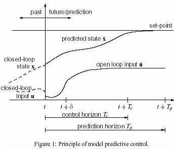
In general, the model predictive control problem is formulated as solving on-line a finite horizon open-loop optimal control problem subject to system dynamics and constraints involving states and controls. 1 shows the basic principle of model predictive control. Based on measurements obtained at time t, the controller predicts the future

Dynamic vehavior of the system over a prediction horizon Tp and determines (over a control horizon Tc < Tp) the input such that a predetermined open-loop performance objective functional is optimized. ,If, there were no disturbances and no model-plant mismatch, and ,if, the optimization problem could be solved for infinite horizons, then one could apply the input function found at time t =0 to the system for all times t > 0. However, this is not possible in general. Due to disturbances and model-plant mismatch,the true system behavior is different from the predicted behavior. In order to incorporate some feedback mechanism,the open-loop manipulated input function obtained will be implemented only until the next measurement becomes available. The time dufference between the recalculation/measurements can vary, however often it is assumed to be fixed, i.e the measurement will take place every sampling tine-units. Using the new measurement at time t
S, the whole procedure - prediction and optimization � is repeated to find to find a new input function with the control and prediction horizons moving forwad.
Notice, hat Figure 1 the input is depicted as arbitrary function of time. As shown in Section 3, for numerical solutions of the open-loop optimal control problem it is often necessary to parameterize the input in an appropriate way.This is normally done by using a finite number of basis functions. E. g. the input could be approximated as piecewise constant over the sampling time .
As will be shown, the calculation of the applied input based on the predicted system behavior allows the inclusion of constraints on states and inputs as well as the optimization of a given cost function. However
since in general the predicted system behavior will differ from the closed-loop one, precaution must be taken to achieve closed-loop stability.
|

