Nonlinear Model Predictive Control

Mathematical Formulation of NMPC

We consider the stabilization problem for a class of system described by the following nonlinear set of differential equations.

Subject to input and state constraints of the form

Where denotes the vector of states and input respectively. The set of feasible input values is denoted by and the set of feasible states is by . we assume that and satisfy the following assumptions: In its simplest form , U and X are given by box constraints of the form: Here are given constant vectors. With respect to the system we additionally assume, that.

Assumption 2 in addition it is locally lipschitz continuous in x. Assumption 3

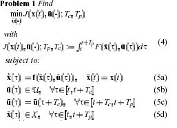
In order to distinguish clearly between the real system and the system model used to predict the �with� the controller, we denote the internal variables in the controller by bar Usually, the finite horizon open-loop optimal control problem described above is mathematically formulated as follows:
Where Tp and Tc are the prediction and the cotrol harizon with Tc <= Tp

The bar denotes internal control variables and is the solution of driven by input with initial condition .the distinction between the real system and the variables in the controller is necessary, since the predicted values, even in the nominal undisturbed case, need not , and in generally will not, be the actual closed-loop values, since the optimal input is recalculated (over a moving finite horizon Tc) at every sampling instance. The bar denotes F in the following called stage cost, specifies the desired control performance that can arise, for example, from economical and ecological considerations. The standard quadratic form is the simplest and most often used one: Where Xs and Us denote given setpoints; Q and R denote positive definite, symmetric weighting matrices. In order for the desired reference to be a feasible solution of problem 1, Us should be contained in the interior of U as already stated in assumption 2 we consider without loss of generality that is the steady state that should be stabilized. Note the initial condition in (5a): the system model used predict the future in the controller is initialized by the actual system state : thus they are assumed to be measured or must be estimated. Equation (5c) is not last step the control horizon. In the following an optimal solution the optimization problem (existence assumed) is denoted by �the open-loop optimal control problem will be solved repeatedly at the sampling instances .,once new measurements are available . the closed-loop is defined by the optimal solution of problem 1 at the sampling instants: The optimal value of the NMPC open-loop optimal control problem as a function of the state will be denoted in the following as value function: The value function plays an important role in the proof of the stability of various NMPC schemes, as it serves as a Lyapunov function candidate.

Properties, Advantages, and Disadvantages of NMPC

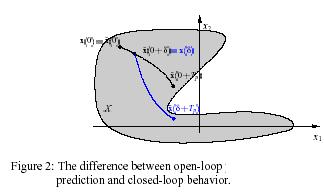
In general one would like to use an infinite prediction and control horizon, i.e. Tc and Tip in problem 1 are set too (5case) to minimize the performance objective determined by the cost However as mentioned, the open-loop optimal control problem 1. that must be solved on-line is often formulated in a finite horizon manner and the input function is parameterized finitely in order to allow a (real-time) numerical solution of the nonlinear open-loop optimal control problem . it clear, that the shorter the horizon the less costly the solution of the on-line optimization problem . thus it is desirable from a computational point of view to implement MPC schemes using short horizons. However, when a finite prediction horizon is used, the actual closed-loop input and state trajectories will differ from the predicted open-loop trajectories, even if no model plant mismatch and no disturbances are present [4] . this fact is depicted in figure 2 where the system can only move inside the shaded area state constraints of the form x = (†) € x are assumed. This makes the key difference between standard control strategies, where the feedback law is obtained a priori and

NMPC where the feedback law is obtained on-line has two immediate consequences. Firstly, the actual goal to compute a feed back such that the performance objective over the infinite horizon of the closed loop is minimized not achieved. In general it is by not means true that a repeated minimization over a finite horizon objective in a receding horizon manner leads to an optimal solution for the infinite horizon problem (with the same stage cost F)[10]. In fact , the two solution differ significantly if a short horizon is chosen.secondly, if the predicted and the actual trajectories