| Sorting |
One of the major applications in computer science is the sorting of information in a table. Sorting algorithms arrange items in a set according to a predefined ordering relation. The most common types of data are string information and numerical information. The ordering relation for numeric data simply involves arranging items in sequence from smallest to largest and from largest to smallest, which is called ascending and descending order respectively.
The items in a set arranged in non-decreasing order are {7,11,13,16,16,19,23}. The items in a set arranged in descending order is of the form {23,19,16,16,13,11,7}
Similarly for string information, {a, abacus, above, be, become, beyond}is in ascending order and { beyond, become, be, above, abacus, a}is in descending order.
There are numerous methods available for sorting information. But, not even one of them is best for all applications. Performance of the methods depends on parameters like, size of the data set, degree of relative order already present in the data etc.
2.3.1 Selection sort
The idea in selection sort is to find the smallest value and place it in an order, then find the next smallest and place in the right order. This process is continued till the entire table is sorted.
Consider the unsorted array,
a[1] a[2] a[8]
The resulting array should be
a[1] a[2] a[8]
One way to sort the unsorted array would be to perform the following steps:
- Find the smallest element in the unsorted array
- Place the smallest element in position of a[1]
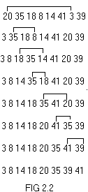
i.e., the smallest element in the unsorted array is 3 so exchange the values of a[1] and a[7]. The array now becomes,
a[1] a[2] a[8]
Now find the smallest from a[2] to a[8] , i.e., 8 so exchange the values of a[2] and a[4] which results with the array shown below,
a[1] a[2] a[8]
Repeat this process until the entire array is sorted. The changes undergone by the array is shown in fig 2.2.The number of moves with this technique is always of the order O(n).
 2.3.2 Insertion sort
Insertion sort is a straight forward method that is useful for small collection of data. The idea here is to obtain the complete solution by inserting an element from the unordered part into the partially ordered solution extending it by one element. Selecting an element from the unordered list could be simple if the first element of that list is selected.
a[1] a[2] a[8]
Initially the whole array is unordered. So select the minimum and put it in place of a[1] to act as sentinel. Now the array is of the form,
a[1] a[2] a[8]
Now we have one element in the sorted list and the remaining elements are in the unordered set. Select the next element to be inserted. If the selected element is less than the preceding element move the preceding element by one position and insert the smaller element.
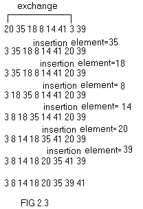
In the above array the next element to be inserted is x=35, but the preceding element is 3 which is less than x. Hence, take the next element for insertion i.e., 18. 18 is less than 35, so move 35 one position ahead and place 18 at that place. The resulting array will be,
a[1] a[2] a[8]
Now the element to be inserted is 8. 8 is less than 35 and 8 is also less than 18 so move 35 and 18 one position right and place 8 at a[2]. This process is carried till the sorted array is obtained.
 The changes undergone are shown in fig 2.3.
One of the disadvantages of the insertion sort method is the amount of movement of data. In the worst case, the number of moves is of the order O(n2). For lengthy records it is quite time consuming.
2.3.3 Merge sort The changes undergone are shown in fig 2.3.
One of the disadvantages of the insertion sort method is the amount of movement of data. In the worst case, the number of moves is of the order O(n2). For lengthy records it is quite time consuming.
2.3.3 Merge sort
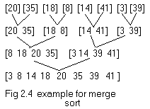
 Merge sort begins by interpreting the inputs as n sorted files each of length one. These are merged pair wise to obtain n/2 files of size two. If n is odd one file is of size one. These n/2 files are then merged pair wise and so on until we are left with only one file. The example in fig 2.4 illustrates the process of merge sort.
As illustrated in the example merge sort consists of several passes over the records being sorted. In the first pass files of size one are merged. In the second pass the size of the files being merged is two. In the ith pass the files being merged will be of size 2i-1. A total of log2n passes are made over the data. Since, two files can be merged in linear time, each pass of merge sort takes O(n) time. As there are log2n passes the total time complexity is O(n log2n). Merge sort begins by interpreting the inputs as n sorted files each of length one. These are merged pair wise to obtain n/2 files of size two. If n is odd one file is of size one. These n/2 files are then merged pair wise and so on until we are left with only one file. The example in fig 2.4 illustrates the process of merge sort.
As illustrated in the example merge sort consists of several passes over the records being sorted. In the first pass files of size one are merged. In the second pass the size of the files being merged is two. In the ith pass the files being merged will be of size 2i-1. A total of log2n passes are made over the data. Since, two files can be merged in linear time, each pass of merge sort takes O(n) time. As there are log2n passes the total time complexity is O(n log2n).
|

